P2P HVDC parametric OHL/UGC transition

This example demonstrates the NetworkBuilder workflow for reusing a cached power-flow solution while sweeping the relative share of overhead line and underground cable in a point-to-point HVDC system.

using PowerImpedance
using CairoMakie
using PowerImpedance.NetworkBuilder: Grid, Gridspace, NetworkState

The P and Q defined here are what is injected into the network.

transmissionVoltage = 380 / sqrt(3)
pHVDC1 = 100
qC1 = 100
qC2 = 100

rho = 100.0
L = 100e3

connections = (
    (node = :B3d, element = :tl1, side = 2, terminal = 1),
    (node = :B3d, element = :c1, side = 2, terminal = 1),
    (node = :B3q, element = :tl1, side = 2, terminal = 2),
    (node = :B3q, element = :c1, side = 2, terminal = 2),
    (node = :B2d, element = :g4, side = 1, terminal = 1),
    (node = :B2d, element = :tl1, side = 1, terminal = 1),
    (node = :B2q, element = :g4, side = 1, terminal = 2),
    (node = :B2q, element = :tl1, side = 1, terminal = 2),
    (node = :B4, element = :ugc, side = 1, terminal = 1),
    (node = :B4, element = :c1, side = 1, terminal = 1),
    (node = :BX, element = :ugc, side = 2, terminal = 1),
    (node = :BX, element = :ohl, side = 1, terminal = 1),
    (node = :B5, element = :ohl, side = 2, terminal = 1),
    (node = :B5, element = :c2, side = 1, terminal = 1),
    (node = :B6d, element = :tl78, side = 1, terminal = 1),
    (node = :B6d, element = :c2, side = 2, terminal = 1),
    (node = :B6q, element = :tl78, side = 1, terminal = 2),
    (node = :B6q, element = :c2, side = 2, terminal = 2),
    (node = :B7d, element = :g1, side = 1, terminal = 1),
    (node = :B7d, element = :tl78, side = 2, terminal = 1),
    (node = :B7q, element = :g1, side = 1, terminal = 2),
    (node = :B7q, element = :tl78, side = 2, terminal = 2)
)

((node = :B3d, element = :tl1, side = 2, terminal = 1), (node = :B3d, element = :c1, side = 2, terminal = 1), (node = :B3q, element = :tl1, side = 2, terminal = 2), (node = :B3q, element = :c1, side = 2, terminal = 2), (node = :B2d, element = :g4, side = 1, terminal = 1), (node = :B2d, element = :tl1, side = 1, terminal = 1), (node = :B2q, element = :g4, side = 1, terminal = 2), (node = :B2q, element = :tl1, side = 1, terminal = 2), (node = :B4, element = :ugc, side = 1, terminal = 1), (node = :B4, element = :c1, side = 1, terminal = 1), (node = :BX, element = :ugc, side = 2, terminal = 1), (node = :BX, element = :ohl, side = 1, terminal = 1), (node = :B5, element = :ohl, side = 2, terminal = 1), (node = :B5, element = :c2, side = 1, terminal = 1), (node = :B6d, element = :tl78, side = 1, terminal = 1), (node = :B6d, element = :c2, side = 2, terminal = 1), (node = :B6q, element = :tl78, side = 1, terminal = 2), (node = :B6q, element = :c2, side = 2, terminal = 2), (node = :B7d, element = :g1, side = 1, terminal = 1), (node = :B7d, element = :tl78, side = 2, terminal = 1), (node = :B7q, element = :g1, side = 1, terminal = 2), (node = :B7q, element = :tl78, side = 2, terminal = 2))

Bus-voltage bounds belong in the builder options used for every case.

builder_options = (;
    voltageBase = transmissionVoltage,
    power_flow = (;
        is_bounded = (;
        bus_voltage = true,
    ),
    )
)

(voltageBase = 219.3931022920578, power_flow = (is_bounded = (bus_voltage = true,),))

x is the fraction of the corridor implemented as underground cable. A 100 m regularization at either endpoint avoids singular zero-length line models.

function ohl_to_ugc(x)
    share = clamp(x, 1e-3, 1 - 1e-3)
    ohl_model = overhead_line(
        length = L * (1 - share),
        conductors = Conductors(
            organization = :flat,
            nᵇ = 2,
            nˢᵇ = 1,
            Rᵈᶜ = 0.0266, rᶜ = 44.8e-3 / 2,
            yᵇᶜ = 18.0, Δyᵇᶜ = 0.0, Δxᵇᶜ = 7.3, Δ̃xᵇᶜ = 0.0,
            dˢᵇ = 0.0,
            dˢᵃᵍ = 6.0
        ),
        groundwires = Groundwires(
            nᵍ = 2,
            Rᵍᵈᶜ = 0.92, rᵍ = 0.0062,
            Δxᵍ = 7.3, Δyᵍ = 7.0, dᵍˢᵃᵍ = 6.0
        ), earth_parameters = (1, 1, rho),
        transformation = true
    )

    ugc_model = cable(
        length = L * share,
        positions = [(-0.5, 1), (0.5, 1)],
        C1 = Conductor(rₒ = 0.02622, ρ = 2.354e-8, μᵣ = 1.035),
        I1 = Insulator(rᵢ = 0.02622, rₒ = 0.06006, ϵᵣ = 2.67, μᵣ = 1.469),
        C2 = Conductor(rᵢ = 0.06006, rₒ = 0.06336, ρ = 2.14e-7, μᵣ = 1.0),
        I2 = Insulator(rᵢ = 0.06336, rₒ = 0.06636, ϵᵣ = 2.3, μᵣ = 1.0),
        C3 = Conductor(rᵢ = 0.06636, rₒ = 0.06651, ρ = 2.826e-8, μᵣ = 1.0),
        I3 = Insulator(rᵢ = 0.06651, rₒ = 0.07256, ϵᵣ = 2.3, μᵣ = 1.0),
        earth_parameters = (1, 1, rho),
        transformation = true
    )

    return (;
        g1 = ac_source(
            setpoint = Setpoint(Vac = transmissionVoltage*sqrt(2),
            Pac = pHVDC1),
            P_min = -2000,
            P_max = 2000,
            Q_max = 1000,
            Q_min = -1000,
            pins = 3,
            transformation = true
        ),

        c1 = only(mmc(Grid; Vᵈᶜ = 640, vDCbase = 640, Vₘ = transmissionVoltage,
            P_max = 1500, P_min = -1500, P = -pHVDC1, Q = qC1, Q_max = 500,
            Q_min = -500,
            occ = PI_control(Kₚ = 0.7691, Kᵢ = 522.7654),
            ccc = PI_control(Kₚ = 0.1048, Kᵢ = 48.1914),
            pll = PI_control(Kₚ = 0.28, Kᵢ = 12.5664),
            q = PI_control(Kₚ = 0.1, Kᵢ = 31.4159),
            dc = PI_control(Kₚ = 6, Kᵢ = 15), timeDelay = 200e-6, padeOrderNum = 5,
            padeOrderDen = 5
        )),

        c2 = only(mmc(Grid; Vᵈᶜ = 640, vDCbase = 640, Vₘ = transmissionVoltage,
            P_max = 1000, P_min = -1000, P = pHVDC1, Q = qC2, Q_max = 1000,
            Q_min = -1000,
            vACbase_LL_RMS = 333, turnsRatio = 333 / 380, Lᵣ = 0.0461, Rᵣ = 0.4103,
            Lₐᵣₘ = 30e-3,
            occ = PI_control(Kₚ = 0.7691, Kᵢ = 522.7654),
            ccc = PI_control(Kₚ = 1 * 0.1048, Kᵢ = 1 * 48.1914),
            pll = PI_control(Kₚ = 0.28, Kᵢ = 12.5664),
            p = PI_control(Kₚ = 1 * 0.1, Kᵢ = 31.4159),
            q = PI_control(Kₚ = 0.1, Kᵢ = 31.4159), timeDelay = 200e-6,
            padeOrderNum = 5, padeOrderDen = 5
        )),

        ugc = ugc_model,
        ohl = ohl_model,

        g4 = ac_source(
            setpoint = Setpoint(Vac = transmissionVoltage*sqrt(2),
            Pac = pHVDC1),
            P_min = -2000,
            P_max = 2000,
            Q_max = 1000,
            Q_min = -1000,
            pins = 3,
            transformation = true
        ),

        tl1 = overhead_line(length = 25e3,
            conductors = Conductors(organization = :flat, nᵇ = 3, nˢᵇ = 1,
                Rᵈᶜ = 0.063,
                rᶜ = 0.015, yᵇᶜ = 30,
                Δyᵇᶜ = 0, Δxᵇᶜ = 10, Δ̃xᵇᶜ = 0, dˢᵇ = 0, dˢᵃᵍ = 10),
            groundwires = Groundwires(
                nᵍ = 2,
                Rᵍᵈᶜ = 0.92,
                rᵍ = 0.0062,
                Δxᵍ = 6.5,
                Δyᵍ = 7.5,
                dᵍˢᵃᵍ = 10
            ),
            earth_parameters = (1, 1, 100), transformation = true),

        tl78 = overhead_line(length = 90e3,
            conductors = Conductors(organization = :flat, nᵇ = 3, nˢᵇ = 1,
                Rᵈᶜ = 0.063,
                rᶜ = 0.015, yᵇᶜ = 30,
                Δyᵇᶜ = 0, Δxᵇᶜ = 10, Δ̃xᵇᶜ = 0, dˢᵇ = 0, dˢᵃᵍ = 10),
            groundwires = Groundwires(
                nᵍ = 2,
                Rᵍᵈᶜ = 0.92,
                rᵍ = 0.0062,
                Δxᵍ = 6.5,
                Δyᵍ = 7.5,
                dᵍˢᵃᵍ = 10
            ),
            earth_parameters = (1, 1, 100), transformation = true)
    )
end

ohl_to_ugc (generic function with 1 method)

The transition is one deterministic Gridspace axis. The axis keeps the OHL and UGC lengths paired, so the study never evaluates an impossible Cartesian product of independent corridor lengths.

function transition_network_space(x_values)
    shares = Grid(collect(x_values))
    return Gridspace{NetworkState}(
        share -> NetworkBuilder.define(
            ohl_to_ugc(share),
            connections;
            options=builder_options,
        ),
        (shares,),
        (:ugc_share,),
    )
end

function transition_peak(response, share)
    magnitude_db = 20 .* log10.(abs.(vec(response.response[1, 1, :])))
    frequencies_hz = real.(response.frequencies) ./ (2π)
    peak_index = argmax(magnitude_db)
    return (;
        ugc_share=share,
        peak_magnitude_db=magnitude_db[peak_index],
        peak_frequency_hz=frequencies_hz[peak_index],
    )
end

function save_transition_animation(study; filename="transition_harmonic_peaks.mp4", fps=8)
    panel = only(study.plot.panels)
    groups = panel.group_order
    CairoMakie.record(study.plot.figure, filename, eachindex(groups); framerate=fps) do frame
        for (index, group) in pairs(groups)
            foreach(plot -> plot.visible[] = index == frame, panel.groups[group])
        end
    end
    foreach(group -> foreach(plot -> plot.visible[] = true, panel.groups[group]), groups)
    return filename
end

function run_transition_study(;
        x_values = 0.0:0.02:1.0,
        frequency_range = (100.0, 5e3, 1000),
        animation_filename = nothing,
        animation_fps = 8,
        display_plot = false
)
    shares = collect(x_values)
    problems = PowerImpedanceProblem(
        transition_network_space(shares);
        nodes=[:B5],
        eliminated_elements=[:c2],
        frequency_range,
    )
    result = compute(
        ParametricProblem(problems),
        Combinatorial(NodalImpedance()),
    )
    labels = ["UGC = $(round(100share; digits=1))%" for share in shares]
    groups = [Symbol("ugc_", replace(string(round(100share; digits=1)), "." => "_"))
              for share in shares]
    plot = only(PowerImpedance.plot(
        result;
        entries=(:B5, :B5),
        labels,
        series_groups=groups,
        title="Impedance at B5 during the OHL/UGC transition",
        figure_size=(950, 700),
        display_plot,
        controls=false,
    ))
    peaks = [transition_peak(response, share)
             for (response, share) in zip(result.values, shares)]
    study = (; result, plot, peaks)
    animation_filename === nothing || save_transition_animation(
        study;
        filename=animation_filename,
        fps=animation_fps,
    )
    return study
end

run_transition_study (generic function with 1 method)

The documentation uses five corridor shares and a reduced frequency grid.

transition_docs = run_transition_study(; x_values=0.0:0.25:1.0, frequency_range=(100.0, 5e3, 160))
transition_docs.plot.figure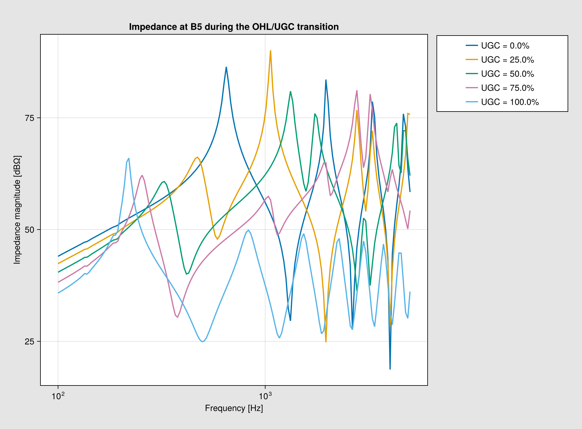

The peak table records the resonance movement seen in the plotted curves.

transition_docs.peaks

5-element Vector{@NamedTuple{ugc_share::Float64, peak_magnitude_db::Float64, peak_frequency_hz::Float64}}:
 (ugc_share = 0.0, peak_magnitude_db = 86.39694221969282, peak_frequency_hz = 648.7633256344882)
 (ugc_share = 0.25, peak_magnitude_db = 90.100074545456, peak_frequency_hz = 1061.190149929239)
 (ugc_share = 0.5, peak_magnitude_db = 80.94713208512204, peak_frequency_hz = 1324.223600336173)
 (ugc_share = 0.75, peak_magnitude_db = 81.1612055125414, peak_frequency_hz = 2770.267466604895)
 (ugc_share = 1.0, peak_magnitude_db = 65.9731997760421, peak_frequency_hz = 219.75110626011713)

Back to Examples